Building an ARIMA Model in Python For Price Forecasting

(There is a notebook with a full example in this repository: https://github.com/GoogleCloudPlatform/training-data-analyst in /ai-for-finance/solution/arima.ipynb)

Building an ARIMA (AutoRegressive Integrated Moving Average) model in Python using the statsmodels library involves several steps. ARIMA is a popular statistical method for time series forecasting. Here’s a step-by-step guide on how to build an ARIMA model for any time-series data, such as stock price prediction. Try focusing on less efficient markets! There will be more alpha to uncover in them.

1. Install and Import Required Libraries

Make sure you have the statsmodels library installed. If not, you can install it using pip:

!pip install statsmodels

Then, import the necessary libraries in your Python script or notebook:

import numpy as np
import pandas as pd
import statsmodels.api as sm
from statsmodels.tsa.arima.model import ARIMA
import matplotlib.pyplot as plt
import yfinance as yf

2. Load and Prepare Your Data

Load your time series data. This data should be a univariate series (i.e., a single series over time). Ensure that the data is in a proper time series format. For this experiment, we’ll use very small timeframes, but using a higher timeframe may make more sense for acquiring/determining stationarity of data. I’m trying a small timeframe in an attempt to discover and exploit inefficiencies that may improve the accuracy of a forecasting model.

# get some small-cap ticker data info a dataframe (note: it must be within the last 60 days for low tf): 

start_date = '2023-12-01'
end_date = '2024-01-01'
interval = '2m'
ticker = 'ACMR'
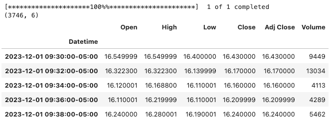
df = yf.download(ticker, start = start_date, end = end_date, interval = interval)
print(df.shape)
df.head()

3. Check for Stationarity

ARIMA requires the time series to be stationary. We know that stock data on high timeframes will tend to trend up and exponentially due to inflation and non-linear economic growth.

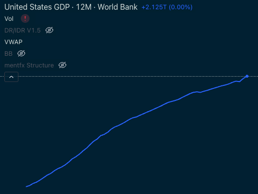
We’ll step back and look at some figures to understand the nature of growth in stock prices over time. Below is US GDP from 1960 to 2024 charted on LOG scale – we can confirm the exponential nature of GDP from this perspective.

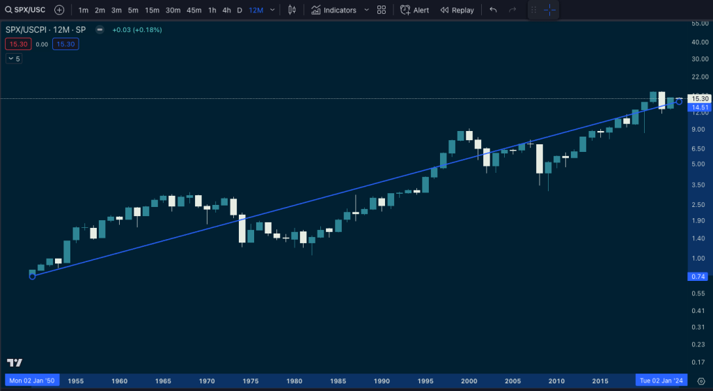
The S&P on LOG scale is still exponential in nominal dollars – in 1932 and 1971 the USD moved away from the gold standard which destabilized the Dollar…

We need to get something closer to real dollars on log scale to find something stable by dividing the S&P by US CPI:

So we can assume stock data is not stationary. Because we’re working on short timeframes, the problem of stationarity is difficult to describe, but we’ll play with the data and see if we can find a good p-value and see what we can come up with.

To gain stationarity, we’ll subtract data from higher timeframes. We can use statistical tests (like the Augmented Dickey-Fuller test) or plot our data to check for stationarity.

from statsmodels.tsa.stattools import adfuller

ts = df['Close']
result = adfuller(ts.dropna())
print('ADF Statistic: %f' % result[0])
print('p-value: %f' % result[1])

# If p-value > 0.05, the series is likely non-stationary

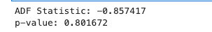
Our p-value is off the charts, so we’ll have to try to stationarize it from higher-timeframe information by resampling and subtracting.


df_hour = df.resample('h').mean()
df_hour = df_hour[['Close']]

# print(df_hour[['Close']].head())

df_hour['hour_ret'] = np.log(df_hour[['Close']]).diff()
# there is one NaN row so drop it
df_hour.dropna(inplace = True)
df_hour['hour_ret'].head()
df_hour.hour_ret.plot(kind='line', figsize = (12, 6));

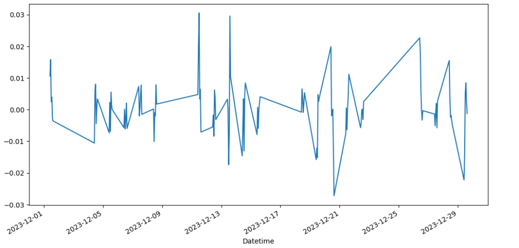
Visually, it looks like we have stationarized our data! We’ll check with the Dickney-Fuller test to be sure:

ts = df_hour['hour_ret']
result = adfuller(ts.dropna())
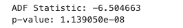
print('ADF Statistic: %f' % result[0])
print('p-value: %e' % result[1])

Note the value is extremely low so I printed it in exponential notation. With p<0.05, we can confirm we have stationary data. We will ignore the close price and use this data.

4. Determine ARIMA Parameters

You need to determine the (p, d, q) parameters for the ARIMA model:

• p: The number of lag observations (AR terms).
• d: The degree of differencing.
• q: The size of the moving average window (MA terms).

You can use plots like the Autocorrelation Function (ACF) and Partial Autocorrelation Function (PACF) to help determine these.

from statsmodels.graphics.tsaplots import plot_acf, plot_pacf
plot_acf(ts)
plt.show()
plot_pacf(ts)
plt.show()

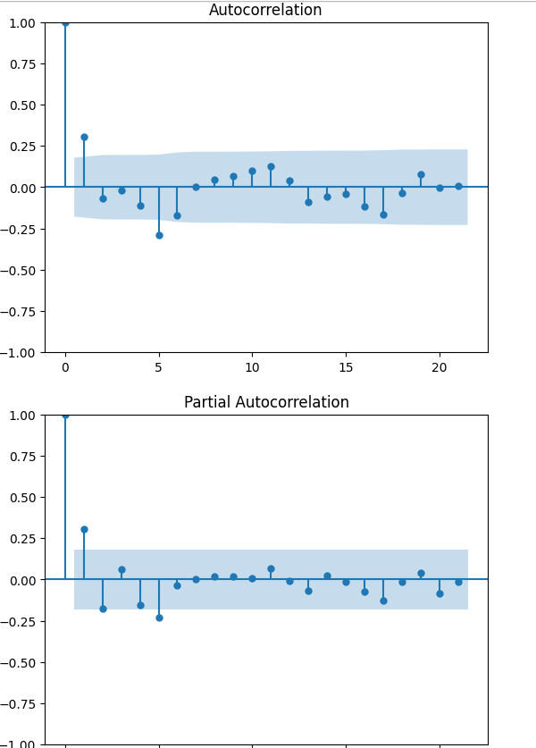
We’ll choose 1 for the ARMA parameters p and q.

5. Fit the ARIMA Model

Now, fit the ARIMA model using the parameters you’ve determined.

# Example: ARIMA with parameters (p=1, d=1, q=1)
model = ARIMA(ts, order=(1, 1, 1))
model_fit = model.fit()

6. Review Model Output

Check the summary of the model to review its performance. Look for the coefficients and their significance, as well as model diagnostics like the AIC (Akaike Information Criterion). A large negative AIC number is a good check. This is not great, but it does have some predictive power.

print(model_fit.summary())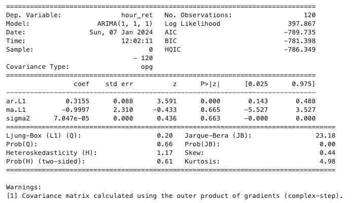

7. Make Predictions

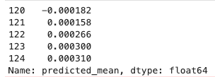
We’ll try to make some predictions into the future and see how the results look. This will predict 5 hours into the future:

# Forecast the next 5 periods
forecast = model_fit.forecast(steps=5)
print(forecast)

8. Evaluate the Model

Evaluate the model’s performance by comparing the forecasts against actual values using metrics like Mean Squared Error (MSE) or Mean Absolute Error (MAE). We can see by visual inspection that our model doesn’t do a great job, but this is also right on the first day of the market year (rotation time!) so we would probably have better luck if we sliced the data at a different point in time.

Remember, choosing the right (p, d, q) parameters is more of an art than a science and often requires experimentation and iteration. It’s also important to ensure your data is appropriately preprocessed and that the model’s assumptions are met for the best results.